A difficult first Machine Learning project
This was the first major assignment in my Machine Learning course, and it was hard to say the least. Feedforward networks brought together many concepts we had only recently learned, especially the mathematics behind forward propagation, loss, gradients, and optimization.
Calculus had also started fading from my memory, which made backpropagation harder to understand. I was not only learning a programming technique. I was rebuilding the mathematical intuition needed to follow how one prediction could influence every earlier weight.
We designed the model around a Keras-like interface because it gave us a familiar way to think about the system. Layers could be added, the model could be compiled and fitted, and the same object supported prediction, evaluation, saving, and loading.
That interface was not only cosmetic. It separated how someone used the network from how the automatic differentiation engine, layers, losses, initializers, and optimizer worked underneath.
Backpropagation met broadcasting
Our three-person team kept ownership clear with little overlap. Julian primarily developed the automatic differentiation Value engine, Sean handled stochastic gradient descent and visualization, and all three of us contributed to the FFNN itself.
My work focused on activation functions, weight initializers, regularization, experiments, and parts of the shared model. I also helped debug the autodiff engine when integration exposed problems that individual components had not revealed.
Backpropagation was the hardest part, especially once tensor broadcasting entered the computation. A forward operation could expand a value across a batch or dimension, but its backward operation had to reduce the resulting gradient into the original shape correctly.
Transpose behavior, reduced gradients, and mismatched dimensions produced calculations that ran but learned the wrong thing. Debugging them forced us to connect the calculus to the exact shapes moving through the program.
The commit history captures the breakthrough better than a formal description: first “it works,” then “IT WORKS BROW,” and finally “accuracy same as sklearn.”
That was the moment our test produced the same result as the library implementation. After struggling with gradients and tensor shapes, seeing the numbers align felt magnificent. It turned backpropagation from a theory we hoped we understood into a system we had evidence was correct.
Initialization was not a small detail
I had underestimated how much initialization could matter. The experiments made the difference impossible to ignore: zero initialization reached only 11.11 percent accuracy, random normal initialization reached 9.79 percent, while Xavier and properly scaled uniform initialization reached roughly 97.29 percent.
Zero initialization also made the symmetry problem concrete. If every neuron begins identically, it receives the same gradient and continues learning the same feature. A network can contain many neurons on paper while behaving as though it has far fewer distinct ones.
Increasing width to 200 neurons produced our best tested result of 97.54 percent, while adding more depth did not automatically help. Additional layers can introduce representational power, but they also introduce more calculations and complexity that the problem may not need.
I did not leave believing that width is always better than depth. The lesson was balance. A model should be broad or deep because the data benefits from it, not because either direction sounds more advanced.
Replacing magic numbers with evidence
A learning rate of 0.5 initially sounded surprisingly large, although papers we had read showed that values in that range could work. Within our limited ten-epoch experiment, it performed well.
Regularization produced the more important surprise. I had treated it almost like a universal improvement, yet L1 reduced accuracy and L2 produced no gain in our test. That result later shaped how I interpreted regularization again in the CNN project.
This project directly influenced the CNN autodiff engine I built in the next assignment. I carried forward the computation-graph model, the lessons about broadcasting, and the habit of checking a from-scratch implementation against an established library.
If I rebuilt the FFNN today, performance would be my first priority. The educational implementation made every mechanism visible, but repeated experiments also made its overhead painful.
The most lasting lesson was that model configuration should not be a collection of unexplained constants. Depth, width, activation, initialization, learning rate, and regularization are all hypotheses about how learning should happen.
Implementing the network taught me how the machinery works. Experimenting with it taught me not to trust magic numbers without evidence.
What stayed with me
- A hyperparameter is a hypothesis, not a magic number.
- Zero initialization can make many neurons learn as one.
- Wider and deeper are different tradeoffs.
- Matching the library turned backpropagation into evidence.
Run it locally
Clone the source repository or download the project ZIP, then run these commands from the project folder.
Explore the complete project
Download the source, assets, and included documentation as a ZIP archive.
Setup
$ python3 -m venv .venv && source .venv/bin/activate
$ pip install numpy scikit-learn matplotlib pandas torch tqdm
Run the worked example
$ cd src
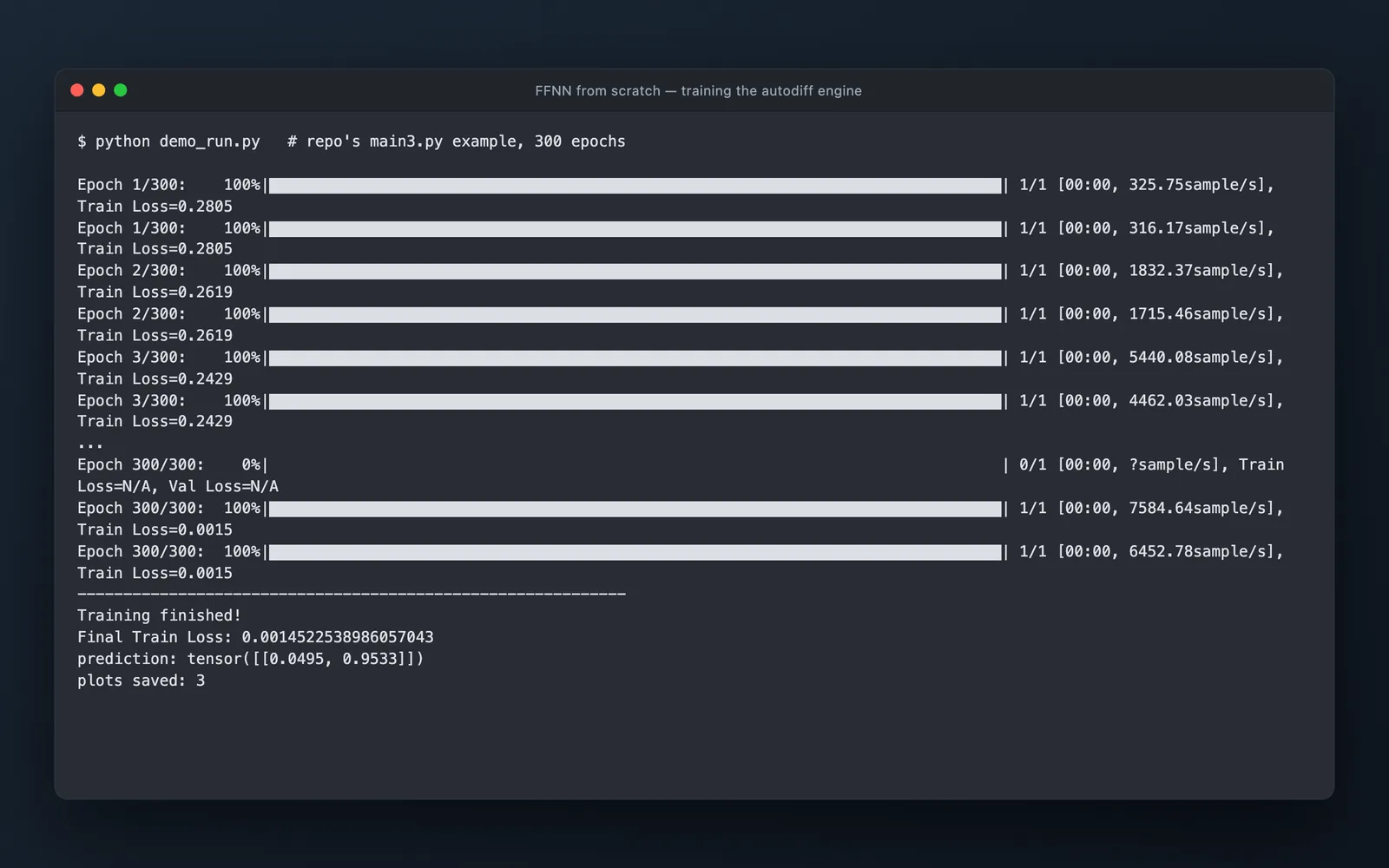
$ python main3.py

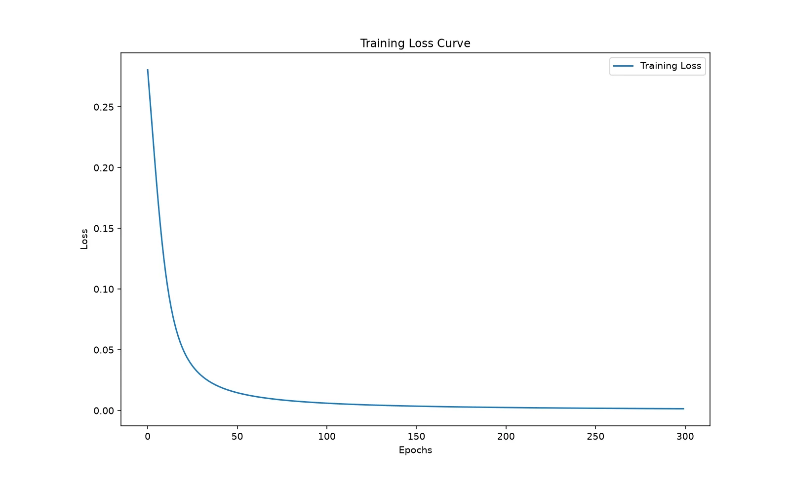
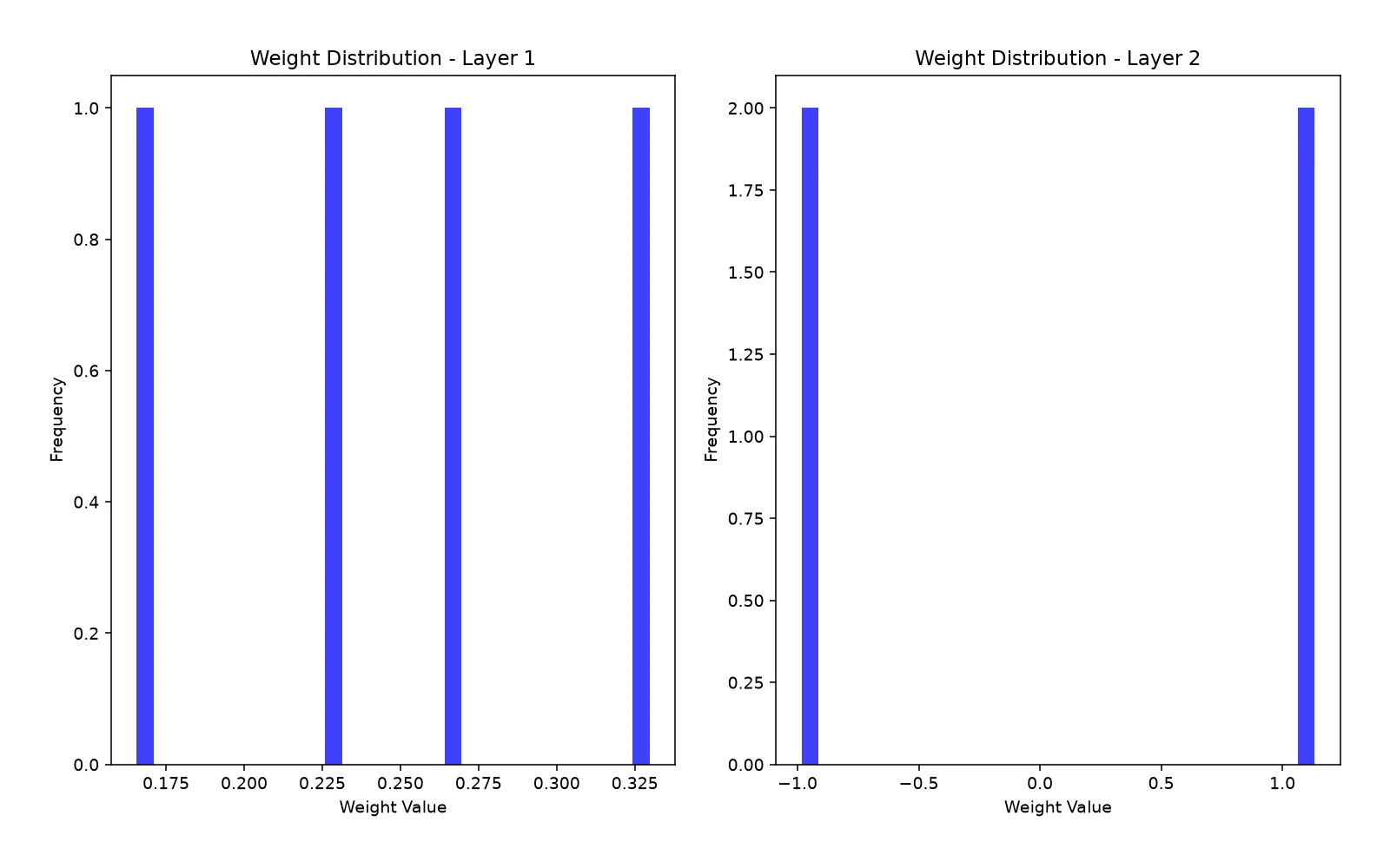
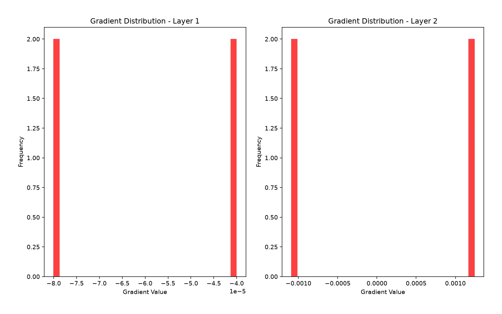
# trains the 2-2-2 sigmoid network from the classic backprop example
Tests
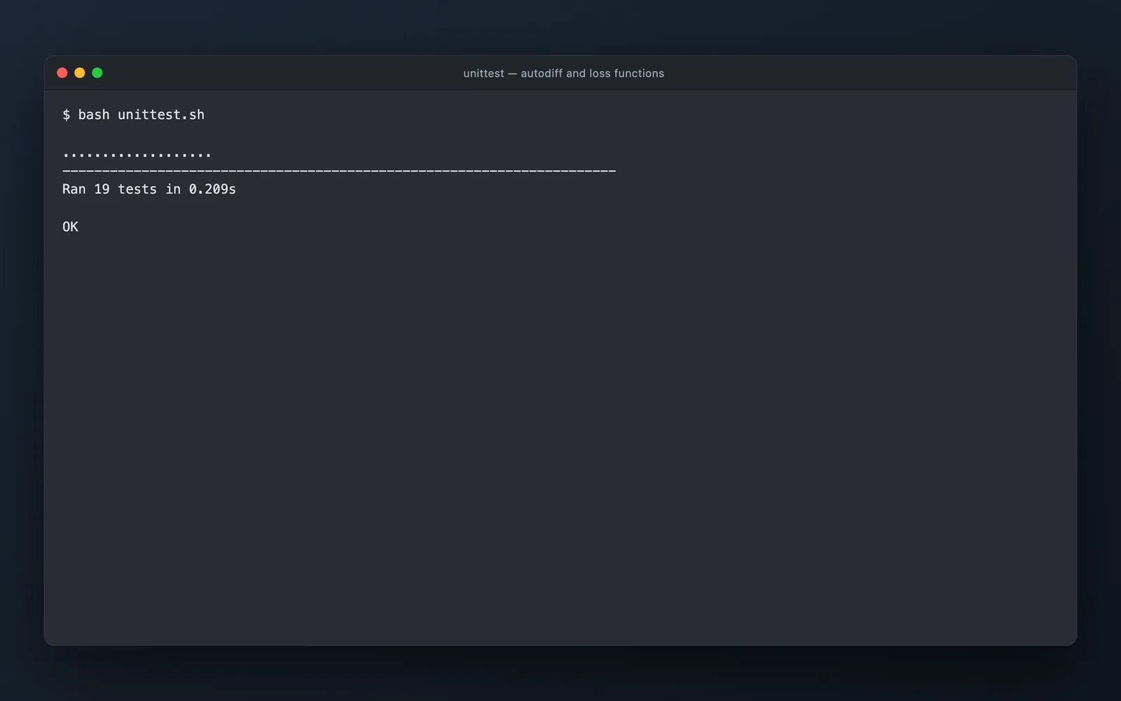
$ bash unittest.sh

# 19 tests across the autodiff engine and the loss functions