CNN from Scratch: Opening the Black Box

This Machine Learning course project was one of the most interesting things I had built because it opened the black box behind neural networks. Until then, I had used the concepts without ever implementing the machinery underneath them.

Our three-person team was assigned one architecture each. I owned the CNN, while my teammates implemented the RNN and LSTM. It was my first time constructing any neural network from scratch.

The assignment required CNN forward and backward propagation, but I chose to build an automatic differentiation engine to support it. Part of the reason was practical. The other part was simply that autodiff sounded cool.

Each operation recorded how its output depended on earlier values. Once the loss was known, the engine could traverse that computation backward and accumulate gradients through the graph.

Making gradients propagate correctly was easily the hardest part. It felt recursive: everything that happened during the forward pass somehow needed to contribute correctly when the calculation traveled in reverse.

For a while, the problem was not subtle. The backpropagation calculation was simply wrong. Tracing shapes, operations, and accumulated gradients through several layers became a long exercise in finding where the backward story stopped matching the forward one.

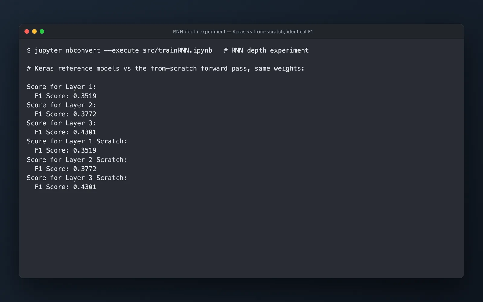
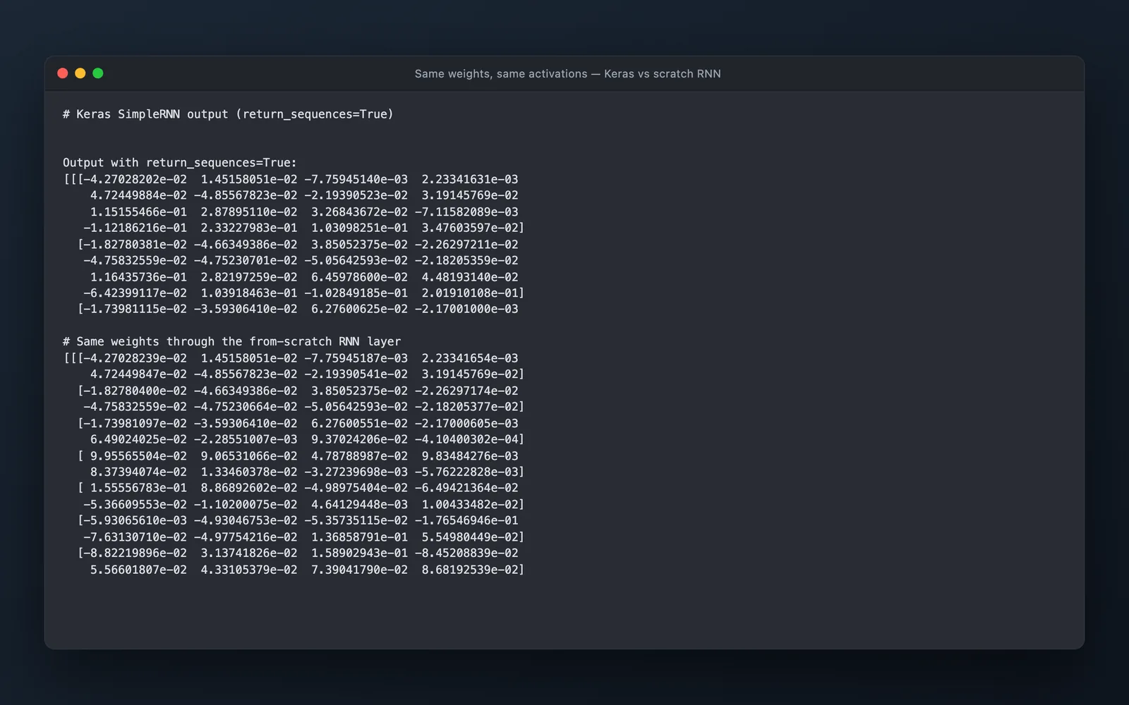
The most satisfying moment was when backpropagation finally produced the correct result. We loaded matching architectures and weights into our implementation and Keras, then compared their outputs on the same inputs.

Seeing both models agree made me happy because it was stronger than watching the loss decrease. It showed that the operations I had written by hand reproduced the behavior of a framework people rely on every day.

We researched architectures that already performed well, so the benefit of adding convolutional layers and filters was broadly expected. Three convolutional layers achieved the best tested Macro F1 score of 0.7229.

Other results were less obvious. A 4 by 4 filter slightly outperformed the other tested sizes. Max pooling also beat average pooling in our context because it preserved the strongest local activation while allowing many weaker, noisy responses to disappear instead of averaging all of them into the result.

That was the value of the experiments. Even when we had an expectation, the implementation gave us a way to test it instead of treating it as a rule.

Testing activation functions was a bonus, but I wanted to push the CNN toward the best result we could get. ReLU achieved the strongest tested accuracy at 97.29 percent on MNIST.

The regularization result was more surprising. I had thought of regularization as something close to a universal improvement, yet it did not help this experiment and sometimes made the result worse. It taught me that a respected technique is still a choice with context, not an accuracy button.

Integrating the CNN, RNN, and LSTM was relatively easy because we designed their shared interfaces with integration in mind from the beginning. Each person could focus on a different internal architecture without making the final project feel like three unrelated programs.

That early agreement mattered. A clean boundary removed much of the integration pain that usually appears when individually correct components finally meet.

Our implementation was slower than the established frameworks, although the gap was not absurd for the experiments we ran. We did not have GPU support, so slow local runs were expected, especially while exploring several configurations.

If I rebuilt it, I would prioritize GPU execution and a cleaner autodiff engine. The current version taught the right ideas, but repeated experiments made every inefficiency visible.

Implementing a CNN from scratch did not make TensorFlow or PyTorch feel ordinary. It made them feel even more magical. Once I understood the amount of gradient bookkeeping beneath a small model, their speed and optimization became more impressive.

The broader lesson was that sophisticated tools and generally useful techniques do not automatically produce the best result. Frameworks, regularization, layer depth, and every other choice still have to fit the problem and the experiment.